Simple scheme for a line-pattern

Many beautiful things arise from very simple rules. That of course neither means that there aren’t beautiful things that really need complicated calculations nor that complicated algorithms cannot result in something truly ugly. But like L-Systems, Newton fractals or Julia sets, the following iteration scheme is easy and yet beautiful to look at.

Rules to create the pattern

The rules for creating the lines are simple and one nice property is that it can very easily be created with paper and pen (unlike for instance Newton fractals). This gives us the perfect starting point to understand the algorithm.

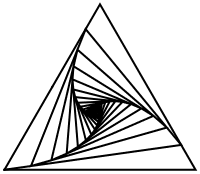
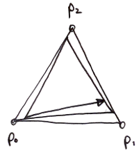Let us first look at a minimal example. Draw three points p0, p1 and p2 so that they shape a triangle and connect them. After that, the iteration is very simple. We start at p0 and draw a line to the point that lies somewhere between p1 and p2. This somewhere is a fixed percentage, so for instance 10% from p1 in the direction of p2. When you reached this new point p3 between p1 and p2, you are drawing the next line starting there and going a position between the next two points. The next two points in this step are now p2 and p0.

Here comes the important point: The next line goes between p0 and the earlier created p3. This means in every step we lose one of the old points by replacing it with a newly calculated point between two existing other points. If this sounds too complicated then try to draw it. It really is very intuitive. In the image above, you can see four iterations of this process and the final position of the pen at the arrow.

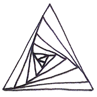
On paper you can just go on and on until the region inside becomes so small that your ending in a point and you have to stop. Surprisingly, the final figure looks really pleasing even though (1) it is not possible to really draw to exact 10% between the next two points and (2) lines may not be exactly accurate. In the second picture you see how it looks for our example with three points. As you might have guessed, this method works of course for more than three points although it becomes increasingly difficult to draw it by hand.

Before we come the the algorithm there is one detail I have skipped: How do we tell the computer when to stop? One easy way is to do the same you did with the pen. We stop when the lines we draw become too short. With this final piece it is possible to write down the algorithm formally

1. Initialization
   • Set starting points \(p_0,\ldots,p_n\)
   • Define a fraction (or percentage) \(0<f<1\)
   • Define a minimal length \(\epsilon\) when we want to stop the iteration
   • Set the current point \(p_{curr}\leftarrow p_0\)
   • Choose \(\epsilon \leftarrow 0.01\) as stopping condition for the iteration
2. Draw a line-strip through the points \(p_0,\ldots,p_n,p_0\) (the final \(p_0\) is required to close the polygon)
3. Choose the next two points \(p_{next1}\) and \(p_{next2}\) that follow \(p_{curr}\).
4. Calculate the new point and update \(p_{next1}\) with the formula \(p_{next1} \leftarrow p_{next1} + f\cdot(p_{next2}-p_{next1})\)
5. Draw a line from \(p_{curr}\) to \(p_{next1}\)
6. Set \(p_{curr}\leftarrow p_{next1}\)
7. If the length of the line-strip \(p_0,\ldots,p_n\) is larger than \(\epsilon\), goto 3.

The above algorithm is a direct procedure that iteratively replaces points in an existing list of points and that draws lines on its way of doing so. By no means it needs to be implemented like this! Rather than simply writing down this recipe, try to think which paradigm would fit best in the language you choose.

The choice of \(\epsilon\) and the condition for stopping the iteration is really not that important. When you draw some figures with a pen, you’ll see that the pattern always contracts and becomes smaller and smaller until you end in a point. Therefore, any measure that tells you how contracted your list of points is or how long the distances between them are will do.

Implementation in Mathematica

For the crucial part of the algorithm, i.e. the handling of the list of points and the calculation of new positions, I’m going to use a simple tail-recursive function. Furthermore, instead of remembering what the current point is, I will always work on the first point of the list. Once I’m finished with it, I’m just sending it off to the back of the list (see line 3) With this trick I’m creating a cyclic list and I don’t need to fiddle around with position pointers:

calcPoints[pts : {pcurr_, pnext1_, pnext2_, rest___}, f_, result_] :=
  calcPoints[
    {pnext1 + f*(pnext2 - pnext1), pnext2, rest, pcurr},
    f,
    {result, pcurr}
  ] /; isNotTooShort[pts];

calcPoints[pts_, _, result_] := Partition[Flatten[result], 2];

The last definition of calcPoints is to return the result when the iteration has stopped. Please note that I’m collecting the points we want for drawing in a nested list in line 6. Therefore the output list of points looks like {p1, {p2, {p3, {p4,...}}}} and in the end I need to flatten it down and re-partition it to recreate the {{x1,y1}, ...} point structure.

Step seven of the algorithm is realized in the test function isNotTooShort which sums up the (squared) distances from point to point and checks whether or not this total length is smaller than the fixed value of \(\epsilon=0.001\).

isNotTooShort[pts_] :=
  Total[SquaredEuclideanDistance @@@ Partition[pts, 2, 1]] > 0.001

With these two definitions, we can try to recreate my hand-drawing by defining three points and plotting the result using a simple Graphics:

pts = {{-1, 0}, {1, 0}, {0, Sqrt[3.0]}};

With[{res = calcPoints[pts, 0.15, {}]},
 Graphics[{Thick, Line[Append[pts, First[pts]]], Line[res]}]
]

That doesn’t look so bad, does it? Once you started doodling around with a pen, you will realize that you can create astonishing effects by simply connecting such figures. After you created one, you start another triangle or rectangle that shares an edge with the former triangle.

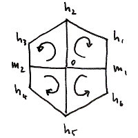
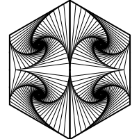
Important is that you don’t forget to play with the drawing direction. If one figure was created drawing clockwise, the neighboring one should be drawn counter-clockwise. We could for instance partition a hexagon into its four quadrants and use the procedure separately on each one.

The scheme for this is visible in the diagram on the right. Corner points of the hexagon can be created in polar coordinates while going one circle in \(2\pi/6\) steps. The midpoints m1 and m2 are then just the mean of their surrounding h points.

o = {0, 0};
h = Table[{Cos[phi + Pi/6], Sin[phi + Pi/6]}, {phi, 0, 2 Pi, Pi/3}];
{m1, m2} = Mean /@ Partition[h[[{1, 6, 3, 4}]], 2];

With[{pts = {
  {o, h[[2]], h[[1]], m1},
  {o, h[[2]], h[[3]], m2},
  {o, h[[5]], h[[4]], m2},
  {o, h[[5]], h[[6]], m1}}},

  Graphics[{Line[calcPoints[#, .1, {}] & /@ pts], Thick, Line /@ pts},
    PlotRange -> {{-1, 1}, {-1, 1}}
  ]
]